This is the first in a series of posts about maximum likelihood methods for fitting statistical models to data. Inspiration for the material comes in large part from Drew Purves who presented something similar. Owen is using Drew’s approach as the basis for this course. Much of the R specific stuff is heavily influenced by Ben Bolker’s excellent book: Ecological Models and Data in R. The goal of this and the following posts includes: learning how to fit to our data more mechanistic models of arbitrary complexity. learning how to do this with ease, confidence, and complete transparency. at some point delving into robust and efficient parameter estimation methods (e.g., MCMC). at some point working out how to switch between frequentist and Bayesian approaches with ease. (Please note that the focus of this post is learning about maximum likelihood methods. R is a only a tool to help that learning, so we avoid putting lots of potentially distracting R code in the post, and rather make it available as a separate file.) Lets start on familiar ground by consider a common statistical approach, linear regression. This involves fitting a model (equation) to the observed data. The equation is:
$$ y = a + bx + norm(0, \sigma) $$
- $ y $ is the observed response variable
- $ x $ is the explanatory variable
- $ a $ is the intercept
- $ b $ is the slope
- $ norm(0, \sigma) $ is the error term.
This is the model we fit to our data. We are trying to find the value of $ a $, $ b $, and $ \sigma $ that fit the data. These are the parameters of the model. How do we find out the values of a and b that give the best regression line? Regression does so by minimizing the sum of squares, which is why we often use the term ‘least squares regression’. We are going to learn how to estimate the parameters of a model by maximising likelihood (instead of minimising least squares). We will start by considering a dataset and model even simpler than linear regression. This example may seem rather trivial. It is. However, better to start simple, with an example adequate to introduce many of the fundamental concepts we need.
Assume we’ve counted the number of individuals in seven replicate quadrats that we’ve placed randomly in a field (don’t ask me why seven quadrats – maybe we left the other three in the lab – who knows). This is our observed data (seven numbers).
Now, the definition of likelihood is $ p(data | model) $
- $ p $ stands for probability
- * data * is the observed data
- $ | $ (the vertical bar) can be read as ‘given the’
- $ model $ = whatever model we like.
That is, $ p(data | model) $ can be read as “the probability of the data given the model”.
In our current example we will assume that individuals in the field are randomly distributed, and therefore that the count in each quadrat comes from a Poission distribution. The Poisson distribution has only one pa- rameter, the mean. This is what we want to estimate. Since this is a trivial example, we can easily find the most likely value of the mean by taking the arithmetic average (mean) of the observed values. We’re not go- ing to do this yet, since the purpose of using this example is illustration of concepts.
So, our model is $ Y_i = Poisson(M) $, where $ Y_i $ is the ith (pronounced eye–eth) observation of the response variable (here the number of individuals counted in the first quadrat) and $ M $ is the mean of the Poisson distribution – this is what we want to estimate.
We want to find the likelihood – $ p(data | model) $ – and so first we calculate the likelihood of each individual observation. The likelihood of the ith observation is,
$$ p(Y_i | M) $$
This is the probability of getting the value $ Y_i $ given the mean $ M $.
So if the first count $ Y_1 = 6 $ and we guess a mean of 7, we can find the probability of $ Y_1 = 6 $ in Excel with: Poisson(6, 7, FALSE) (why false?). Or in R using dpois(6, 7)
If you do either of these you will find that the probability of observing a 6 given a Poisson distribution with mean 7 is about 0.15.
We do this for each value of the response variable, log the probabilities, and then add them up. Lets do this in Excel, using the worksheet ‘eg1’ in this Excel spreadsheet. Here is a screen grab of the worksheet:
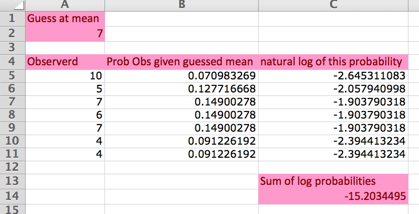
The first column (from row 4 down) is the data, the second is the probability of each data point given the mean (look at the formula to see the call to the Excel Possion function). The third column is the log (base e; ln) of the probabilities (i.e., the log-likelihood. Often this is just called the likelihood, but we should try to always use the term log-likelihood, for accuracy. At the bottom of column C is the sum of the log-likelihoods. Cell A2 contains our guess of the mean of the observed data.
- Look at the formulas in the cells to check they are what you expect.
- Try changing the guess of the mean and see what happens to the sum of the log probabilities.
By changing the guess of the mean (cell A2 in the worksheet ‘eg1’) you change the log-likelihood. The challenge is to find the value of the mean that will minimise the log-likelihood (= maximise the likelihood). This value (estimate) of the mean is called the maximum likelihood estimate. We are interested in maximising the likelihood, or equivalently, minimising it (make as close to zero as possible). The more negative the sum of log likelihood the worse the model (guess of the mean) is. (Read this paragraph while playing with the Excel worksheet, until you are sure you get it. It is very important.)
(By the way, we log the probabilities for a few reasons, including that computers often have problems deal- ing with very small numbers.)
By playing with the guess of the mean in cell A2 of the Excel worksheet, you may have found that a value close to 6 minimises the log-likelihood (makes it closest to zero, i.e., least negative). You have just obtained a maximum likelihood estimate of the parameter of this model.
Now take a look at the R script file eg1.r. This shows how you can do with R what you just did with Excel.
Of course, we don’t want to have to guess the mean, look at the log-likelihood, guess again, and look at the log-likelihood again, and so on. We want the computer to do the work. In the R file is some script that makes a vector of guesses of the mean, loops through these, and records the log-likelihood. Then we can plot the value of the log-likelihood versus the guess of the mean.
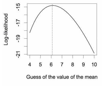
The maximum of this curve is the maximum likelihood. It is achieved when the guess of the mean has the val- ue of 6.1, where the vertical dashed line is drawn. The log-likelihood here is -14.821. This curve is also know as the likelihood profile.
How did we do? Our guess was 6.1 and the actual mean is 6.143, with a log-likelihood of -14.820. Not bad then!
Question for you: What should we change in the R script to get a more accurate estimate of the mean?
Now, this is important. If we suspected our observed data were poisson distributed, and we wanted to mod- el that data in R, we might easily decide to use the generalised linear model funtion glm and specify a pois- son distribution (family=poisson). The code to do this would look something like, glm(n ~ 1, family=poisson) where n is the response variable that here is the number of individuals in each of the quadrats.
This model is in the R script previously mentioned, and the coefficient (estimated parameter / mean) is 1.8153. Not the mean that we found (6.1). This is because specifying a poisson distribution (family=poisson) means that a log link function is used. So we have to un-log the coefficient to get the actual value… exp(1.8153) = 6.1428. Good.
What else can we do with this simple example? Let’s figure out for ourselves the AIC (Akaike Information Cri- teria) of our model. The definition of AIC is,
$$ AIC = -2*L + 2*n $$
Where L is the log-likelihood and p is the number of parameters (only one, the mean, in our model). Our log-likelihood was -14.82117, so AIC = 31.64. The AIC given by the glm function is 31.64 also. Great.
How does glm work? How does it find the mean? It tries many guesses of the mean and sees which gives the maximum likelihood, just like we did in the R script that made the graph above. However, glm uses a search method that is a bit smarter than ours (I think it calls the function optim which by default uses the Nelder-Mead search algorith, but this is not too important now). What is important is to realise that glm is just searching around the parameter space looking for a maximum likelihood. It tries to go uphill on the likelihood profile. When it can’t go uphill any more, it knows it’s reached the maximum likelihood.
You should now be able to have a good go at answering these questions:
- What are parameters?
- What is a variable?
- What is likelihood?
- What does this mean p(data| model)?
- How can we maximise likelihood.
- What is the maximum likelihood estimate of a parameter?
- What is a likelihood profile?