Inspiration for the following from from Richard McElreath’s Statistical Rethinking book, and some of the code comes from here: https://bookdown.org/ajkurz/Statistical_Rethinking_recoded/multivariate-linear-models.html#masked-relationship
Let us think about the question of how the response variable y is related to two explanatory variables x1 and x2.
First we make a dataset in which we know the relationships because we specify them: we make y = x1 - x2. Before this, we create x1 and x2 and make them correlated…
rm(list=ls())
library(tidyverse)
library(patchwork)
set.seed(141)  # setting the seed makes the results reproducible
N   <- 100   # number of observations
rho <- .8      # correlation between x_pos and x_neg
dd <-
  tibble(x1 = rnorm(N),
         x2 = rnorm(N, rho*x1, sqrt(1 - rho^2)),
         y     = rnorm(N, x1 - x2))
A quick look at the dataset… three numeric <dbl> variables.
glimpse(dd)
## Observations: 100
## Variables: 3
## $ x1 <dbl> 0.51435972, -0.11277738, 0.06434006, -0.65524480, 0.50172420, -0.8…
## $ x2 <dbl> 0.929913616, 0.824215658, -0.060507248, -0.182433894, 1.952874568,…
## $ y  <dbl> -1.927385720, -0.028922502, 0.405574747, 0.629677348, -2.459065811…
Figure 1 shows the three scatterplots on can make. Importantly, we see little evidence of the relationship between y and x1, or between y and x2 that we know exist. We can clearly see the correlation between the two explanatory variables x1 and x2.
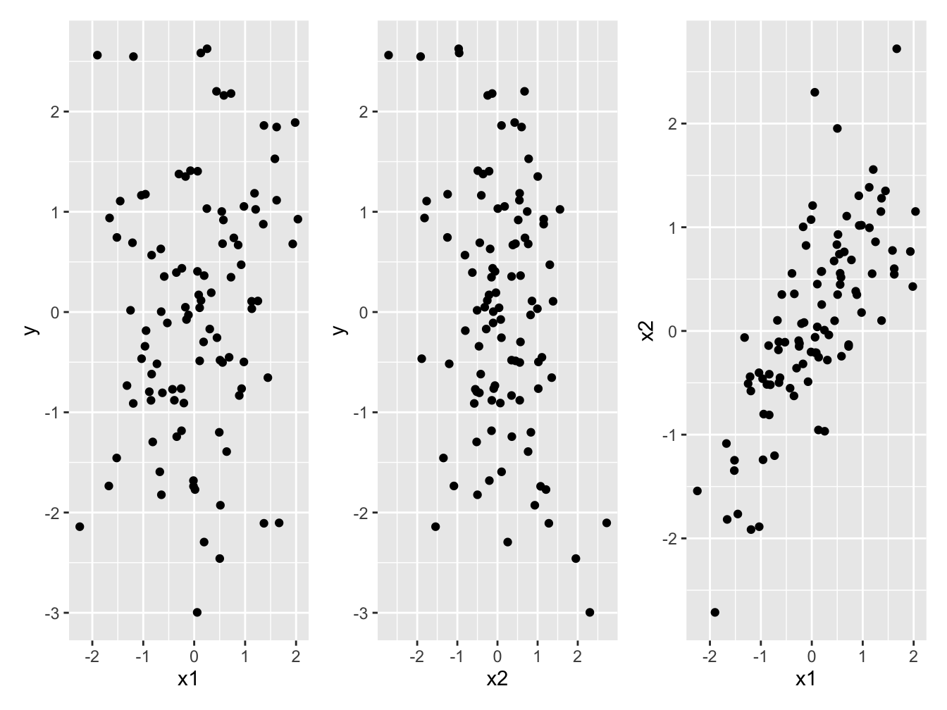
Figure 1: (a and b) Little evidence of a relationship between the response variable *y* and either of the two explanatory variables *x1*, or *x2*. (c) Strong correlation between the two explanatory variables *x1* and *x2*
To reveal the relationship between y and x1 we need to control for the variation in x2. One way to do this is to divide the data into subsets in each of which there is relatively little variation in x2. With the following code we add a variable to the data set that contains categories of variation in x2. I.e. we cut the variation in x2 into 10 groups, and put the names of these groups in a new variable:
dd <- mutate(dd,
            x2_cut = cut(x2, 10))
Figure 2, in particular the panels with more observations, clearly shows the positive relationships that we know exist. Great! Have a go at making an analogous plot while controlling for variation in x1. (By the way, we have more data in the middle, because x2 is normally distriuted.)
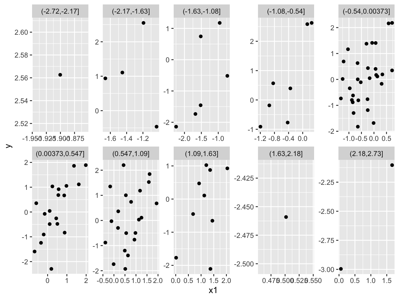
Figure 2: The positive relationship between the response variable (*y*) and one of the explanatory variables (*x1*) is visible because each facet shows a relatively small range of variation in the other explanatory variable (*x2*).
Another way to control for variation in each explanatory variable while “viewing” the relationship of the response variable with the other is multiple regression. Below we see very strong evidence of the positive relationship between y and x1 and negative between y and x2, and that estimated coefficients (slopes) are not different from the real ones (1). Whereas the univariate regression show much weaker evidence of any relationships, and estimated coefficients are poorly estimated.
Multiple regression is, in effect, doing what we did when we cut up the data and plotted parts of it that contained little variation in the other variable.
mod_x1x2 <- lm(y ~ x1 + x2, data = dd)
summary(mod_x1x2)
##
## Call:
## lm(formula = y ~ x1 + x2, data = dd)
##
## Residuals:
##      Min       1Q   Median       3Q      Max
## -2.27190 -0.64723 -0.04082  0.68422  2.73434
##
## Coefficients:
##             Estimate Std. Error t value Pr(>|t|)
## (Intercept)  0.07772    0.09878   0.787    0.433
## x1           1.13521    0.15776   7.196 1.31e-10 ***
## x2          -1.26254    0.16259  -7.765 8.44e-12 ***
## ---
## Signif. codes:  0 '***' 0.001 '**' 0.01 '*' 0.05 '.' 0.1 ' ' 1
##
## Residual standard error: 0.983 on 97 degrees of freedom
## Multiple R-squared:  0.3996,	Adjusted R-squared:  0.3872
## F-statistic: 32.27 on 2 and 97 DF,  p-value: 1.801e-11
mod_x1 <- lm(y ~ x1, data = dd)
summary(mod_x1)
##
## Call:
## lm(formula = y ~ x1, data = dd)
##
## Residuals:
##      Min       1Q   Median       3Q      Max
## -3.02457 -0.72337  0.00238  0.79139  2.95465
##
## Coefficients:
##             Estimate Std. Error t value Pr(>|t|)
## (Intercept)  0.01596    0.12473   0.128    0.898
## x1           0.21467    0.13186   1.628    0.107
##
## Residual standard error: 1.245 on 98 degrees of freedom
## Multiple R-squared:  0.02633,	Adjusted R-squared:  0.0164
## F-statistic:  2.65 on 1 and 98 DF,  p-value: 0.1067
mod_x2 <- lm(y ~ x2, data = dd)
summary(mod_x2)
##
## Call:
## lm(formula = y ~ x2, data = dd)
##
## Residuals:
##      Min       1Q   Median       3Q      Max
## -2.79342 -0.95557 -0.02311  0.94306  2.39910
##
## Coefficients:
##             Estimate Std. Error t value Pr(>|t|)
## (Intercept)  0.06106    0.12167   0.502  0.61689
## x2          -0.38332    0.13218  -2.900  0.00461 **
## ---
## Signif. codes:  0 '***' 0.001 '**' 0.01 '*' 0.05 '.' 0.1 ' ' 1
##
## Residual standard error: 1.211 on 98 degrees of freedom
## Multiple R-squared:  0.07904,	Adjusted R-squared:  0.06964
## F-statistic:  8.41 on 1 and 98 DF,  p-value: 0.004606